FREEWAYS
LEVEL OF SERVICE
Density is the
primary determinant of LOS on a freeway.
In other words, it is the Performance
Criterion for freeways. LOS
thresholds for a basic freeway segment are defined in terms of density as
follows:
LOS Density
Range (pc/mi/ln)
A 0–11
B > 11–18
C > 18–26
D >
26–35
E > 35–45
F > 45
The
relationship between density, level of service, speed, and flow is shown in the
following graph:
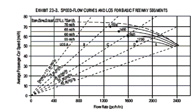
Notice that
capacity = 2400 passenger cars per hour (per lane) in this figure. The flow rate in this figure is represented
by the variable Vp and the free flow speed in this figure is designated as
FFS. If we know, Vp and FFS we can use
this graph to determine both the density and level of service. Or we can use Vp and FFS to find the Speed
(S) from this graph and then calculate density using the standard
speed/flow/density equation D = Vp / S (a rearrangement of q = S x D where q is
the same as Vp). In either case, we
must first determine FFS and Vp to calculate density and LOS.
DETERMINING FREE FLOW SPEED
The Free Flow
Speed (FFS) is the mean speed of passenger cars measured during low to moderate
flows (up to 1300 pc/h/ln). For a
specific segment of freeway, speeds are virtually constant in this range of
flow rates. Two methods can be used to
determine the FFS of a basic freeway segment: field measurement and estimation with guidelines provided in this
chapter. The speed study should be conducted at a location that is
representative of the segment when flows and densities are low (less than 1300
pc/h/ln). Weekday off-peak hours are
generally good times to observe low to moderate flow rates.
The speed
study should measure the speeds of all passenger cars or use a systematic sample
(e.g., every 10th passenger car). The speed study should measure passenger-car speeds
across all lanes. A sample of at least 100 passenger-car speeds should be obtained.
Any speed measurement technique that has been found acceptable for other types
of traffic engineering speed studies may be used.
The average of
all passenger-car speeds measured in the field under low-to-moderate-volume
conditions can be used directly as the FFS of the freeway segment. This speed reflects the net effect of all
conditions at the study site that influence speed, including those considered
in this method (lane width, lateral clearance, interchange density, and number
of lanes) as well as others such as speed limit and vertical and horizontal
alignment. Speed data that include both passenger cars and heavy vehicles can
be used for
level terrain or moderate downgrades but should not be used for rolling or mountainous
terrain.
If field
measurement of FFS is not possible, FFS can be estimated indirectly on the basis
of the physical characteristics of the freeway segment being studied. The
physical characteristics include lane width, number of lanes, right-shoulder
lateral clearance, and interchange density:
BFFS
= 70 mph for urban freeways and 75 mph for rural freeways.
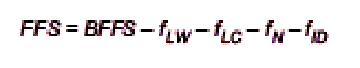
The first
adjustment (fLW) relates to the effect of lane widths on Free Flow
Speed. Base conditions for a two-lane
highway require lane widths of 12-ft or greater.
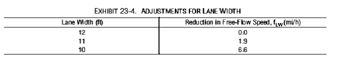
The second adjustment (fLC) relates to the effect of
right shoulder lateral clearance on Free Flow Speed, and is dependent on the
number of lanes in one direction.
Considerable
judgment must be used in determining whether objects or barriers along the
right side of a freeway present a true obstruction. Such obstructions may be continuous, such as retaining walls,
concrete barriers, or guardrails, or may be non-continuous, such as light
supports or bridge abutments. In some
cases, drivers may become accustomed to certain types of obstructions, in which
case their influence on traffic flow may be negligible.
The third adjustment (fN) relates to the effect of the number of lanes in one direction on Free Flow Speed. It is only used for urban and suburban freeways, not rural freeways.
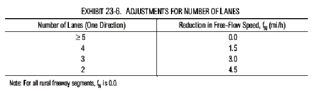
In determining
number of lanes, only mainline lanes should be considered. HOV lanes should not be included.
The fourth
adjustment (fID) relates to the effect of interchange density on
Free Flow Speed.
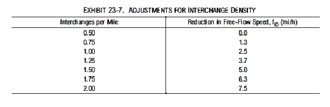
The base
interchange density is 0.5 interchange per mile, or 2 mile interchange spacing. Base free-flow speed is reduced when
interchange density becomes greater than this. Interchange density is determined over a 6 mile segment of freeway
(3 mile upstream and 3 mile downstream) in which the freeway segment is
located.
DETERMINING DEMAND FLOW RATE
(Vp)
The hourly
flow rate must reflect the influence of heavy vehicles, the temporal variation
of traffic flow over an hour, and the characteristics of the driver population. These effects are reflected by adjusting
hourly volumes or estimates, typically reported in vehicles per hour (veh/h),
to arrive at an equivalent passenger car flow rate in passenger cars per hour
(pc/h). The equivalent passenger-car flow rate is calculated using the heavy vehicle
and peak hour adjustment factors and is reported on a per lane basis
(pc/h/ln). Four adjustments must be made to hourly demand
volumes (V) to arrive at the equivalent passenger car flow rate (VP). These adjustments are the PHF, number of lanes (N) in one direction,
the heavy vehicle adjustment factor (fHV), and the driver population
adjustment factor (fp). These adjustments are applied
using the following equation:

Heavy
Vehicle Adjustment (fHV)
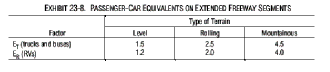
Adjustment for the presence of heavy vehicles in the traffic stream applies to two types of vehicles: trucks and RVs. Buses should not be treated as a separate type of heavy vehicle but should be included with trucks. The heavy-vehicle adjustment factor requires two steps. First, the passenger-car equivalency factors for trucks (ET) and RVs (ER) for the prevailing operating conditions must be found.
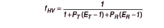
Once values
for ET and ER have been determined, the adjustment factor
for heavy vehicles (fHV) is computed using the following equation
where PT is the percentage of trucks in the traffic stream
(expressed as a decimal) and PR is the percentage of RV’s in the
traffic stream (also expressed as a decimal):
Driver
Population Adjustment (fP)
The traffic
stream characteristics that are the basis of this methodology are representative
of regular drivers in a substantially commuter traffic stream or in a stream in
which most drivers are familiar with the facility. It is generally accepted that traffic streams with different
characteristics (e.g., recreational drivers) use freeways less efficiently. The adjustment factor fp is used to reflect
this effect. The values of fp range
from 0.85 to 1.00. In general, the analyst should select 1.00, which reflects
commuter traffic (i.e., familiar users), unless there is sufficient evidence
that a lower value should be applied.